Understand common-used Evaluations Metrics for Binary Classification

This blog is based on the content of:

[1] Olson, David L., and Dursun Delen. Advanced data mining techniques. Springer Science & Business Media, 2008.

[2] Géron, Aurélien. Hands-on machine learning with Scikit-Learn, Keras, and TensorFlow: Concepts, tools, and techniques to build intelligent systems. O'Reilly Media, 2019.

[3] Davis, Jesse, and Mark Goadrich. "The relationship between Precision-Recall and ROC curves." Proceedings of the 23rd international conference on Machine learning. 2006.

[4] Schütze, H., Manning, C. D., & Raghavan, P. (2008). "Chapter 8: Evaluation in information retrieval"  Introduction to information retrieval (Vol. 39, pp. 234-265). Cambridge: Cambridge University Press.

---------------------------------------------------

This blog aims to summarize the common used evaluations metrics for binary classification with particular emphasis on class imbalance problems. 

Let's start by understanding the confusion matrix.

Confusion Matrix

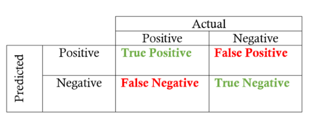
Positive/Negative: based on prediction result

        Positive: predict Positive

        Negative: predict Negative 

    True/False: based on actual label

True: the prediction is correct

        False: the prediction is wrong

To understand each term in confusion matrix, we first look at Positive/Negative according to the prediction result, add True/False in the front then according to the actual label:  

- True Positive (TP):  Predict Positive and the prediction is Correct (Positive in real case)

- False Positive (FP): Predict Positive but the prediction is False (Negative in real case)

- True Negative (TN):  Predict Negative and the prediction is Correct (Negative in real case)

- False Negative (FN):  Predict Negative but the prediction is False (Positive in real case)

Accuracy

Accuracy is the proportion of true results among the total number of cases examined. It is used when the classes are well balanced.

•  Accuracy Paradox.  High Accuracy might be too crude to be useful.  For example, in a dataset which contains 99 normal samples and 1 anomaly. If a model predicted all as ‘normal’. Then this model has a 99% accuracy but useless to detect anomaly.Precision and Recall are more useful in class imbalance (skewed dataset) cases.

Precision

The proportion of predicted Positives that is truly positive.

• Precision VS Accuracy. Precision focuses only on the instances that are predicted Positive. Accuracy considers both instances that are predicted Positive and Negative. 

As the denominator of precision is all positive predictions, a trivial way to have perfect precision is to make only one single positive prediction and ensure it is correct (Precision =1/1 = 100%). So prediction is typically used with recall.

Recall

The proportion of actual Positives that is correctly classified.

Precision-Recall Curves

• Threshold. Classifiers compute a score [class probability] for each instance and if that score is greater than threshold, it assigns the instance to the positive class, otherwise it assigns the instance to the negative class. So we we calculate the precision and recall of a classifier, we are actually calculating precision and recall of this classifier in a certain threshold (by default is 0.5).

By varying the threshold value, we obtains a set of Precision/Recall pairs. Plotting all the Precision/Recall pairs in to a graph we get a Precision-Recall curve.

Precision-Recall curve [1]

One functionality of the Precision-Recall curve is to find the threshold that best serves our need. 

F1-Score

It is convenient to combine Precision and Recall into a single metric ‘F1-score’.  

F1-score is the ‘Harmonic Mean’ of Precision and Recall. Compared to ‘Arithmetic Mean’, ‘Harmonic Mean’ penalizes more the case when one’s value is much lower than another.  

As a result, to get a high F1-score, both Precision and Recall need to be high.

However, depending on the application scenario, the highest F1-score might not be the best solution.  For example, in anomaly detection, you might want to detect all the actual anomalies (high recall) even though many normal instances might be misclassed to the anomaly class (low precision).

Apart from the Precision-Recall curve, Receiver Operating Characteristics (ROC) curve is another permanence evaluation technique for classification models.  

ROC curves have long been used in signal detection theory to depict the trade-off between hit rate and false alarm rates of classifiers.  Compared with the Precision-Recall curve, the ROC curve is not influenced by the skew in the class distribution, which will be demonstrated later. 

A few metrics to be introduced before reaching ROC curves:

Sensitivity and Specificity

Sensitivity:

Specificity:

    

The nominator of Specificity is True Negative. However, in many cases, we care more about false alarms, which means how many actual negative instances are incorrectly classified as positive.  

Therefore False Positive Rate (FPR) = 1- Specificity, is often used.

True Positive Rate (TPR) and False Positive rate(FPR)

True Positive Rate:

False Positive Rate:

TPR and FPR are not influenced by the skew in class distribution

From a Conditional Probability point of view:

Assume :

• 1 corresponds to Positive class 
• 0 correspond to Negative class. 
• X is the predicted class label
• Y is the actual class label .

Then:

• Precision = P(Y=1|X=1)
• FPR= Recall = Sensitivity = P(X=1|Y=1)
• TPR = 1 - Specificity = 1 -P(X=0|Y=0)

Both FPR and TPR are probabilities conditioned on the true class label, which means that their values remain the same regardless of what P(Y=1) is. Thus they are not affected by the distribution of the true class label.  However, as Precision is probabilities conditioned on the estimated class label, it will vary when the dataset is skewed. 

ROC(Receiver Operating Characteristic)

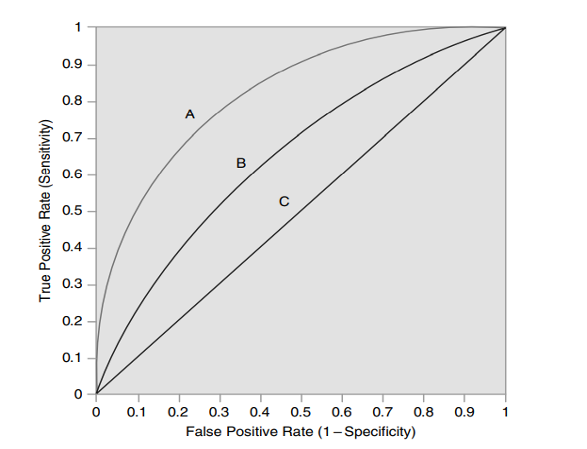
The ROC curve is plotted by traversing all thresholds with TPR on the Y axis and FPR on the X axis.

Several points to note in the graph:

• Lower left (0,0): Never issuing a positive classification.  (Assigning all to negative class)
• Upper right (1,1): Unconditionally issuing positive classification. (Assigning all to positive class)
• Upper left (0,1): Perfect Classification.  More the curve is close to the upper left point (0,1), the better the classifier is.  So in this ROC graph, A is the most performant classifier, followed by B , and then C [2].

ROC curve [2]

Classifiers that appear on the lower left hand side of a ROC curve could be considered as ‘conservative’: making positive classification only with strong evidence so they have low false alarm. 

Classifiers that appear on the upper right of a ROC curve could be considered as ‘liberal’: making positive classification with weak evidence to classify all the actual positives correctly and often have a high false positive rate [2]. 

In order to compare the model’s performance regardless of threshold, one may want to reduce the ROC measures to a single scalar metric: AUC.

• AUC. AUC is the abbreviation of Area Under Curve. Here AUC stands for the AUC of ROC curves but similarly there is also AUC for P-R curves.  The value of AUC curves varies in [0,1], which a perfect classifier gets a value of 1. The diagonal line (C in the graph) stands for the strategy of randomly guessing a class (AUC = 0.5).  As ROC curves are the measures regardless of skew in class distribution, AUC is a measure of models’ classification performance regardless of both skew in the class distribution and threshold. 

• Visualization.I strongly encourage you to check this article who did a amazing visualization about ROC curve: https://www.spectrumnews.org/opinion/viewpoint/quest-autism-biomarkers-faces-steep-statistical-challenges/

ROC vs Precision-Recall Curve 

Assume :

• 1 corresponds to Positive class 
• 0 correspond to Negative class. 
• X is the predicted class label
• Y is the actual class label .

P-R curve consists of:

• Precision = P(Y=1|X=1)
• Recall = FPR = Sensitivity = P(X=1|Y=1)

ROC curve consists of:

• TPR = 1 - Specificity = 1 - P(X=0|Y=0)
• FPR = Recall = Sensitivity = P(X=1|Y=1)

It is not difficult to find that both two curves share Recall (=TPR), however, P-R curves focus only on Positive class (it is more useful when one is much more interested in Positive class than Negative class) but ROC curves consider both positive and negative classes. 

 Actually, according to [3]:

‘‘ROC curve present an overly optimistic view of an algorithm’s performance if there is a large skew in the class distribution’’

However, the ROC curve remains the same regardless of the class distribution, which means that the ROC curve could show the model general performance at a variety of class distributions (check: https://www.spectrumnews.org/opinion/viewpoint/quest-autism-biomarkers-faces-steep-statistical-challenges/). And of course, if false positive rate is a huge concern, the ROC curve would be more indicative. 

More relationships between two curves are illustrated in the same paper [3]:

‘‘For any dataset, the ROC curve and PR curve for a given algorithm contain the same points. This equivalence leads to the surprising theorem that a curve dominates in ROC space if and only if it dominates in PR space. [...] Finally, we show that an algorithm that optimizes the area under the ROC curve is not guaranteed to optimize the area under the PR curve.’’

-------------------

Thank you so much for reading my blog! If you have any thoughts or opinions on the topic, I would love to hear from you in the comments below. See you soon !

Github: https://github.com/TianyiDataScience

Linkedin: https://www.linkedin.com/in/tianyi-li-v

-------------------